In-Memory Datasets¶

Generic Unigrid Data¶

The most common example on in-memory or “generic” data is that of data that is generated in memory from the currently running script or notebook. In this example, we’ll just create a 3-D array of random floating-point data:

arr = rand(64,64,64)

To load this data into YT, we need to associate it with a field. The data dictionary consists of one or more fields, each consisting of a tuple of an Array and a unit string. Then, we can call load_uniform_grid:

data = Dict()
data["density"] = (arr, "g/cm**3")
bbox = [-1.5 1.5; -1.5 1.5; -1.5 1.5]
ds = YT.load_uniform_grid(data, [64,64,64]; length_unit="Mpc", bbox=bbox, nprocs=64)

load_uniform_grid takes the following arguments and optional keywords:

• data : This is a dict of numpy arrays, where the keys are the field names
• domain_dimensions : The domain dimensions of the unigrid
• length_unit : The unit that corresponds to code_length, can be a string, tuple, or floating-point number
• bbox : Size of computational domain in units of code_length
• nprocs : If greater than 1, will create this number of subarrays out of data
• sim_time : The simulation time in seconds
• mass_unit : The unit that corresponds to code_mass, can be a string, tuple, or floating-point number
• time_unit : The unit that corresponds to code_time, can be a string, tuple, or floating-point number
• velocity_unit : The unit that corresponds to code_velocity
• magnetic_unit : The unit that corresponds to code_magnetic, i.e. the internal units used to represent magnetic field strengths.
• periodicity : A tuple of booleans that determines whether the data will be treated as periodic along each axis

This example creates a yt-native dataset ds that will treat your array as a density field in cubic domain of 3 Mpc edge size and simultaneously divide the domain into nprocs = 64 chunks, so that you can take advantage of the underlying parallelism.

The optional unit keyword arguments allow for the default units of the dataset to be set. They can be:

• A string, e.g. length_unit="Mpc"
• A tuple, e.g. mass_unit=(1.0e14, "Msun")
• A floating-point value, e.g. time_unit=3.1557e13

In the latter case, the unit is assumed to be cgs.

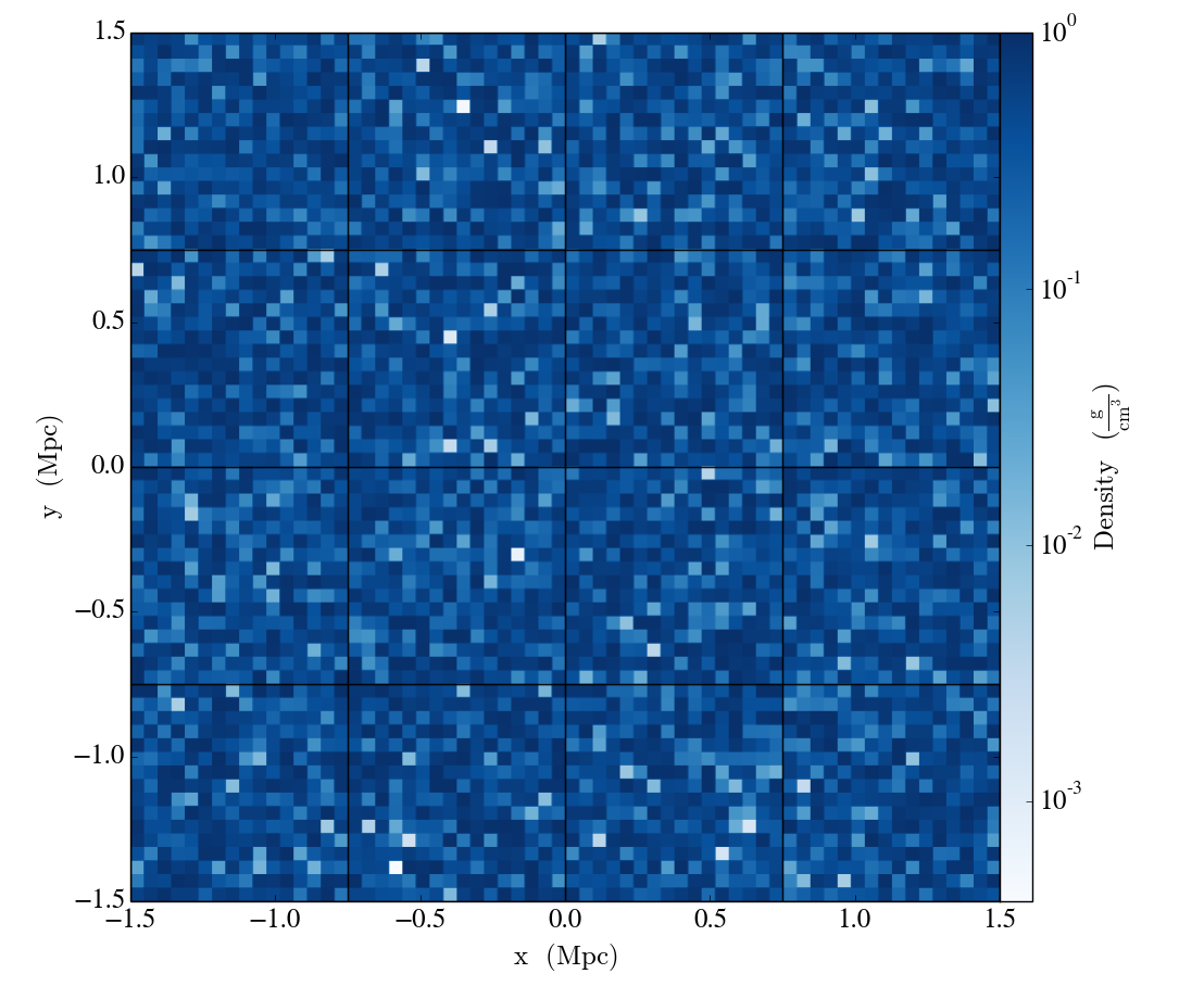
The resulting ds functions exactly like a dataset like any other YT can handle–it can be sliced, and we can show the grid boundaries:

slc = YT.SlicePlot(ds, "z", ["density"])
slc.set_cmap("density", "Blues")
slc.annotate_grids(cmap=nothing)
YT.show_plot(slc)

Particle fields are detected as one-dimensional fields. The number of particles is set by the number_of_particles key in data. Particle fields are then added as one-dimensional Arrays in a similar manner as the three-dimensional grid fields:

arr = rand(64,64,64)
posx_arr = 3*rand(10000)-1.5
posy_arr = 3*rand(10000)-1.5
posz_arr = 3*rand(10000)-1.5
data = Dict()
data["density"] = (arr, "Msun/kpc**3")
data["number_of_particles"] = 10000
data["particle_position_x"] = (posx_arr, "code_length")
data["particle_position_y"] = (posy_arr, "code_length")
data["particle_position_z"] = (posz_arr, "code_length")
bbox = [-1.5 1.5; -1.5 1.5; -1.5 1.5]
lu = (1.0,"Mpc")
mu = (1.0,"Msun")
ds = YT.load_uniform_grid(data, [64,64,64]; length_unit=lu, mass_unit=mu, bbox=bbox, nprocs=4)

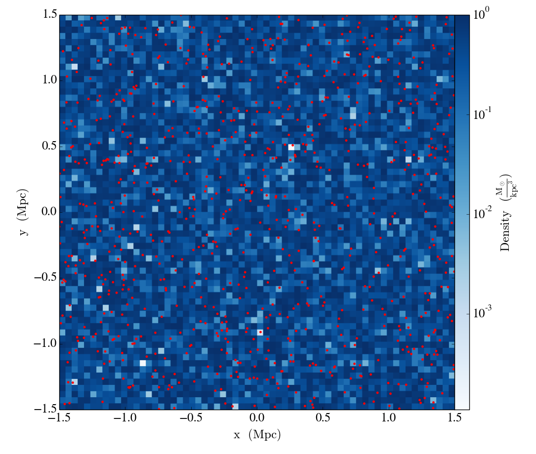
In this example only the particle position fields have been assigned. number_of_particles must be the same size as the particle arrays. If no particle arrays are supplied then number_of_particles is assumed to be zero. Take a slice, and overlay particle positions:

slc = YT.SlicePlot(ds, "z", ["density"])
slc.set_cmap("density", "Blues")
slc.annotate_particles(0.25, p_size=12.0, col="Red")
YT.show_plot(slc)

Generic AMR Data¶

In a similar fashion to unigrid data, data gridded into rectangular patches at varying levels of resolution may also be loaded into YT. In this case, a list of grid dictionaries should be provided, with the requisite information about each grid’s properties. This example sets up two grids: a top-level grid (level == 0) covering the entire domain and a subgrid at level == 1.

grid_data = [
    ["left_edge"=>[0.0, 0.0, 0.0],
     "right_edge"=>[1.0, 1.0, 1.0],
     "level"=>0,
     "dimensions"=>[32, 32, 32]],
    ["left_edge"=>[0.25, 0.25, 0.25],
     "right_edge"=>[0.75, 0.75, 0.75],
     "level"=>1,
     "dimensions"=>[32, 32, 32]]
   ]

We’ll just fill each grid with random density data, with a scaling with the grid refinement level.

for g in grid_data
    g["density"] = rand(g["dimensions"]...) * 2^g["level"]
end

Particle fields are supported by adding 1-dimensional arrays to each grid and setting the number_of_particles key in each grid‘s dict. If a grid has no particles, set number_of_particles = 0, but the particle fields still have to be defined since they are defined elsewhere; set them to empty Float64 Arrays:

grid_data[1]["number_of_particles"] = 0 # Set no particles in the top-level grid
grid_data[1]["particle_position_x"] = Float64[] # No particles, so set empty arrays
grid_data[1]["particle_position_y"] = Float64[]
grid_data[1]["particle_position_z"] = Float64[]
grid_data[2]["number_of_particles"] = 1000
grid_data[2]["particle_position_x"] = 0.5*rand(1000)+0.25
grid_data[2]["particle_position_y"] = 0.5*rand(1000)+0.25
grid_data[2]["particle_position_z"] = 0.5*rand(1000)+0.25

We need to specify the field units in a field_units Dict:

field_units = ["density"=>"code_mass/code_length**3",

Then, call load_amr_grids:

ds = YT.load_amr_grids(grid_data, [32, 32, 32]; field_units=field_units)

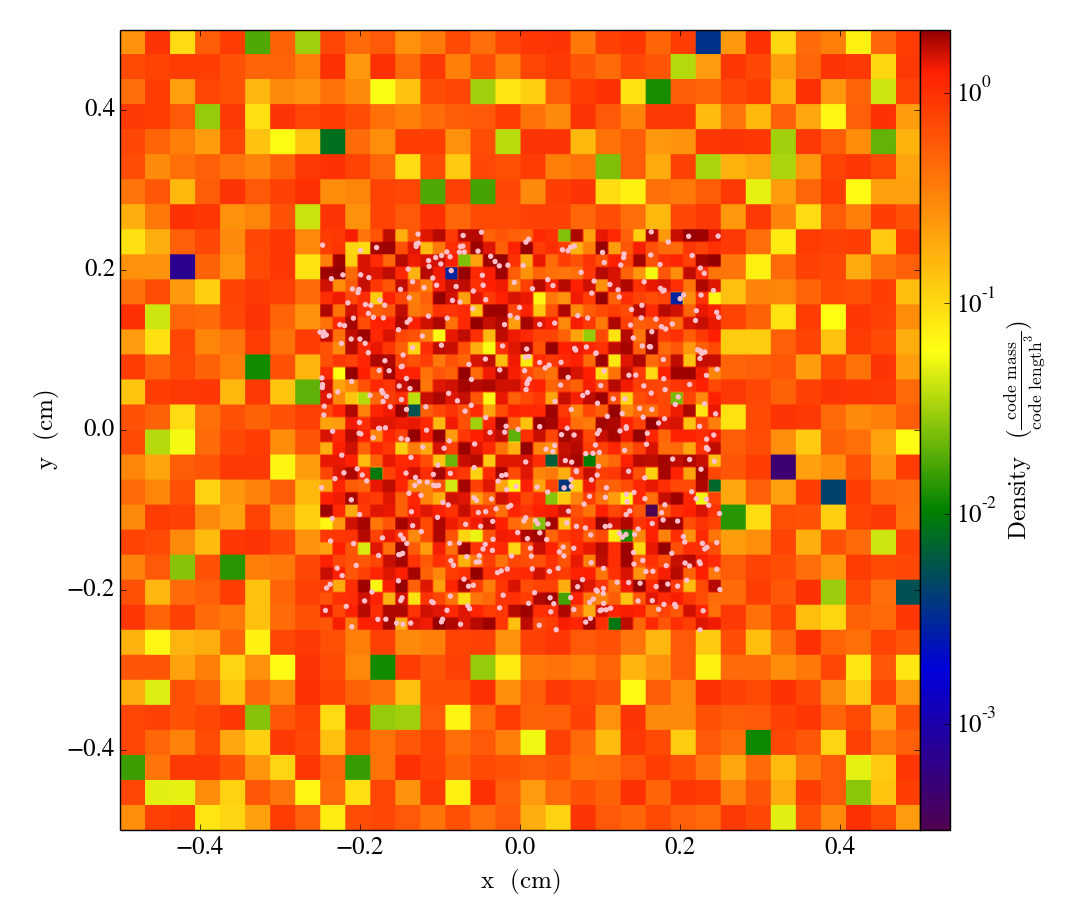
load_amr_grids also takes the same keywords bbox and sim_time as load_uniform_grid. We could have also specified the length, time, velocity, and mass units in the same manner as before. Let’s take a slice:

slc = YT.SlicePlot(ds, "z", ["density"])
slc.annotate_particles(0.25, p_size=15.0, col="Pink")
YT.show_plot(slc)

Generic Particle Data¶

This example creates a fake in-memory particle dataset and then loads it as a YT dataset using the load_particles function.

Our “fake” dataset will be Arrays filled with normally distributed random particle positions and uniform particle masses. Since real data is often scaled, we arbitrarily multiply by 1e6 to show how to deal with scaled data.

The load_particles function accepts a dictionary populated with particle data fields loaded in memory as Arrays:

n_particles = 5000000
data = Dict()
data["particle_position_x"] = 1.0e6*randn(n_particles)
data["particle_position_y"] = 1.0e6*randn(n_particles)
data["particle_position_z"] = 1.0e6*randn(n_particles)
data["particle_mass"] = ones(n_particles)

To hook up with yt‘s internal field system, the dictionary keys must be 'particle_position_x', 'particle_position_y', 'particle_position_z', and 'particle_mass', as well as any other particle field provided by one of the particle frontends.

The load_particles function transforms the data dictionary into an in-memory YT Dataset object, providing an interface for further analysis with YT. The example below illustrates how to load the data dictionary we created above.

bbox = 1.1*[minimum(data["particle_position_x"]) maximum(data["particle_position_x"]);
    minimum(data["particle_position_y"]) maximum(data["particle_position_y"]);
    minimum(data["particle_position_z"]) maximum(data["particle_position_z"])]

ds = YT.load_particles(data, length_unit="pc", mass_unit=(1e8, "Msun"), n_ref=256, bbox=bbox)

The length_unit and mass_unit are the conversion from the units used in the data dictionary to CGS. I’ve arbitrarily chosen one parsec and \(10^8 M_\odot\) for this example.

The n_ref parameter controls how many particle it takes to accumulate in an oct-tree cell to trigger refinement. Larger n_ref will decrease poisson noise at the cost of resolution in the octree.

Finally, the bbox parameter is a bounding box in the units of the dataset that contains all of the particles. This is used to set the size of the base octree block.

This new dataset acts like any other YT Dataset object, and can be used to create data objects and query for YT fields. This example shows how to access “deposit” fields:

ad = YT.AllData(ds)
cic_density = ad["deposit", "all_cic"]
nn_density = ad["deposit", "all_density"]
nn_deposited_mass = ad["deposit", "all_mass"]
particle_count_per_cell = ad["deposit", "all_count"]

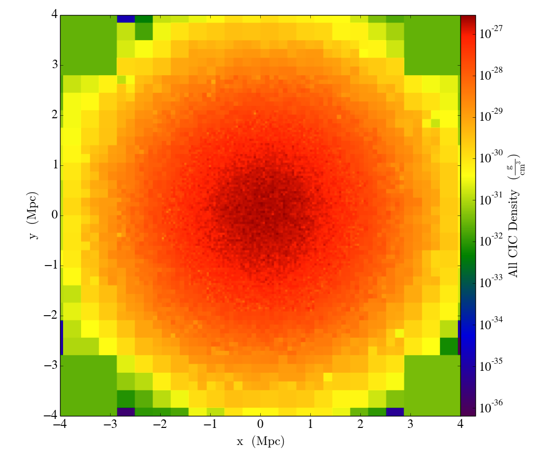
Finally, we’ll slice through the "all_cic" deposited particle field:

slc = YT.SlicePlot(ds, 2, ("deposit", "all_cic"))
slc.set_width((8, "Mpc"))
YT.show_plot(slc)