Plotting and Images
Plots
YT provides an interface to two of the most common plotting routines in yt: SlicePlot and ProjectionPlot:
function SlicePlot(ds::Dataset, axis, fields; center="c", args...)

function ProjectionPlot(ds::Dataset, axis, fields; center="c", data_source=nothing, args...)
Unlike other methods in YT, these return the native yt Python-based objects. This is mainly for convenience; it allows one to use all of the annotation and plot modification methods that hang off these objects. The API for these objects is the same as it is in yt, which can be found in the yt plotting documentation.
We’ll illustrate the plotting functionality with a SlicePlot as an example:
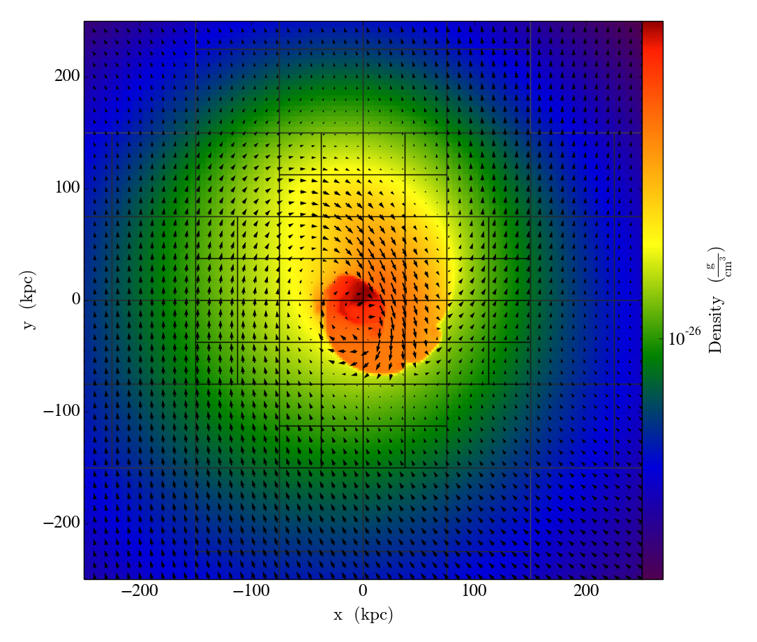
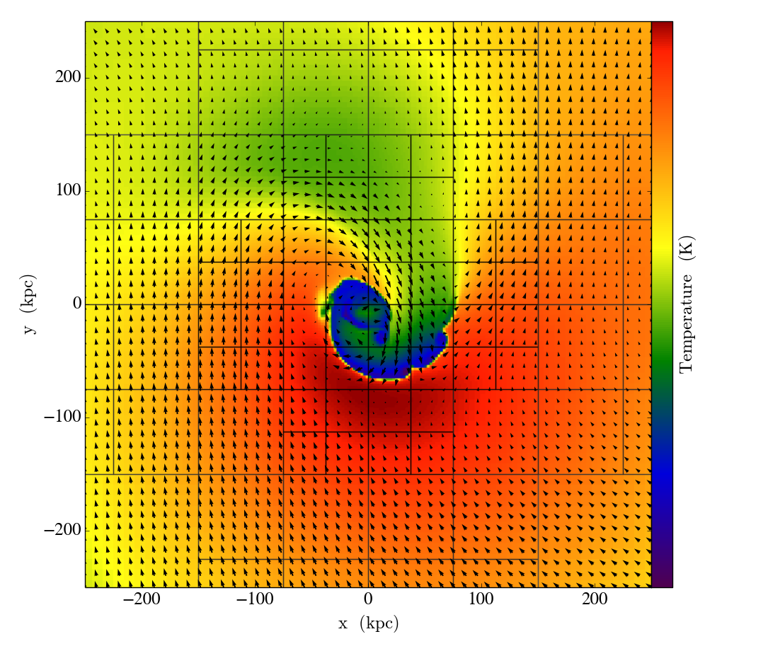
julia> slc = YT.SlicePlot(ds, "z", ["density","temperature"], width=(500.,"kpc"))

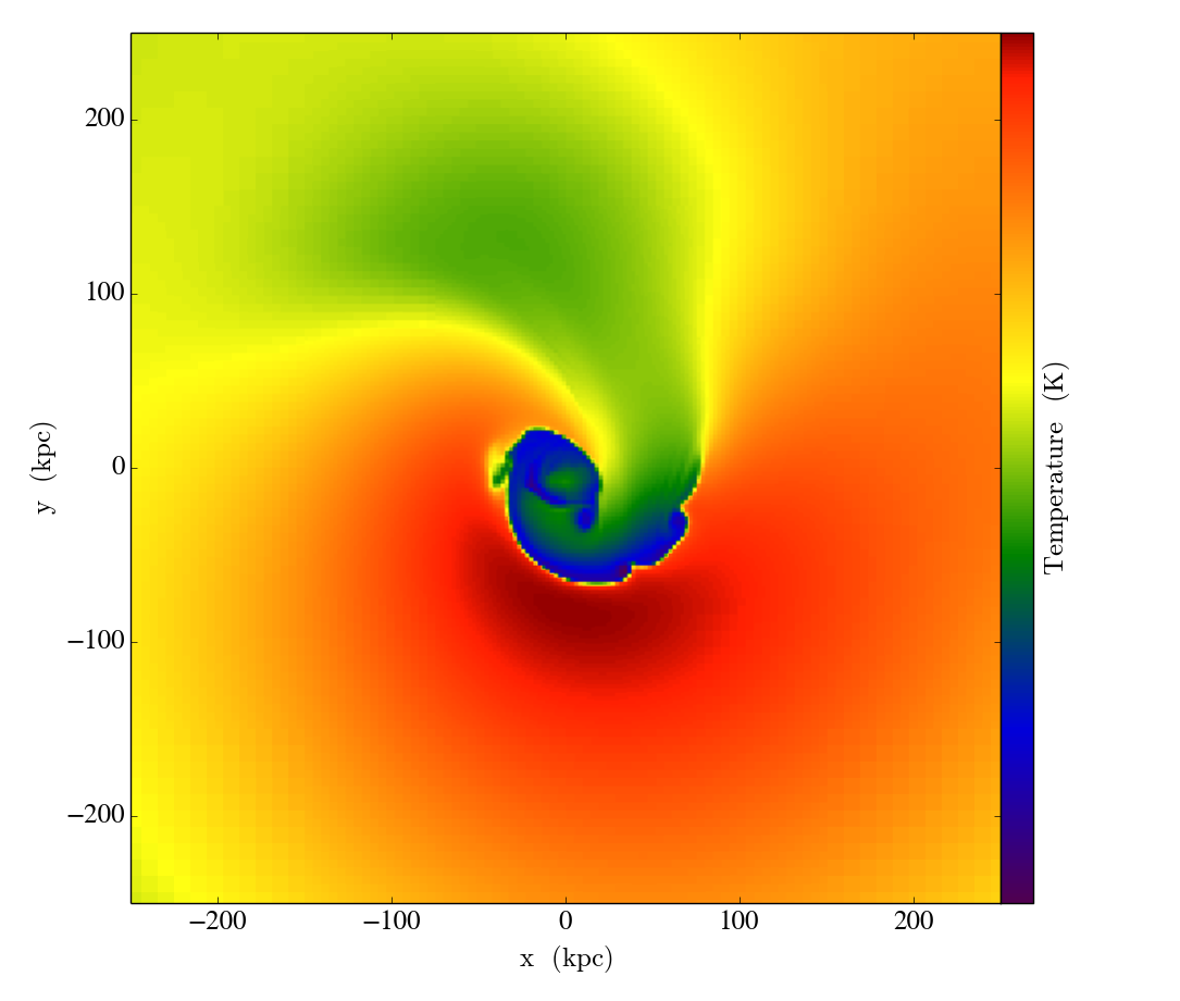
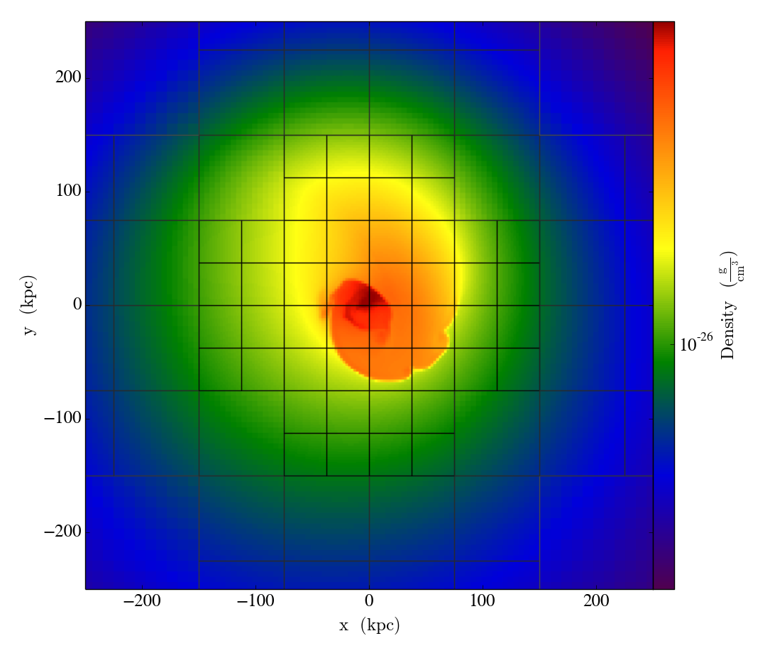
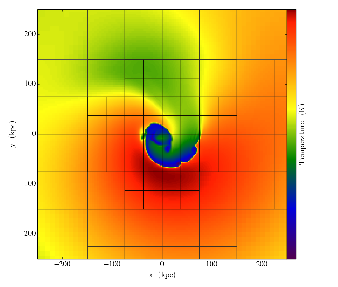
which produces a SlicePlot PyObject of the fields “density” and “temperature”, along the “z” axis. The optional argument width has been used to zoom on on the central 500 kpc of the domain. The SlicePlot object has available to it all of the methods for annotating the plot that one would have access to in yt. For example, one can annotate grids:
julia> slc.annotate_grids()
or velocity vectors:
julia> slc.annotate_velocity()
Logging can be set for specific fields:
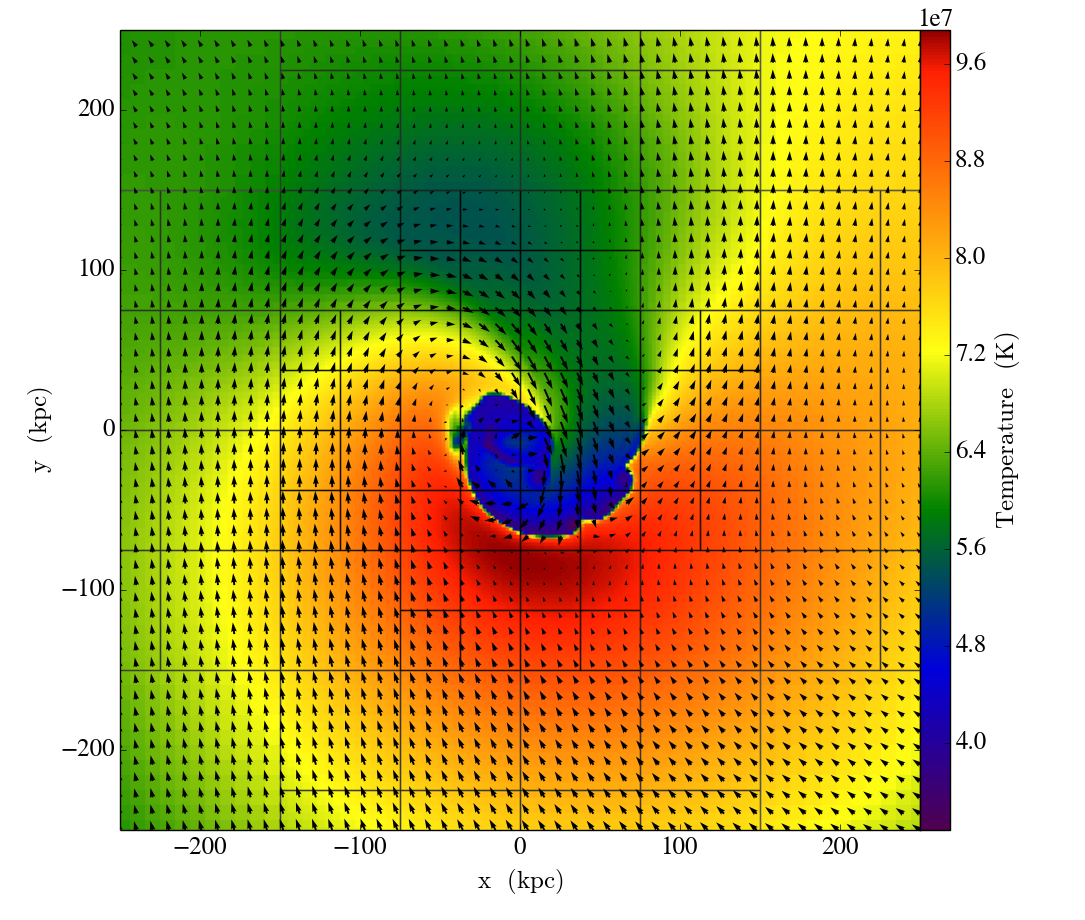
julia> slc.set_log("temperature", false)
or the colormap can be changed:
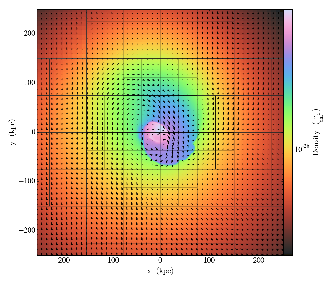
julia> slc.set_cmap("density", "kamae")
To save a plot:
julia> slc.save("my_awesome_plot.png")
If one is in the IJulia notebook, the show_plot method can be used to display the plot inline:
julia> YT.show_plot(slc)
The full set of options for these plots can be found in the yt plotting documentation.
Images
To create a raw 2D image from a Slice or Proj object, one can create a FixedResolutionBuffer object using the to_frb method:
function to_frb(cont::Union(Slice,Proj), width::Length,
                  nx::Union(Integer,(Integer,Integer)); center=nothing, height=nothing,
                  args...)
where cont is the Slice or Proj object, width is the width of the plot, nx is the resolution of the image, center is the center of the image (defaults to the center of the cont), and height is the height of the image (defaults to the width). The resolution nx can either be a single value or a tuple of two values, depending on how you want to set the width and height. This is an example of how to create a FixedResolutionBuffer from a Slice:
julia> slc = YT.Slice(ds, "z", 0.0)
YTSlice (sloshing_nomag2_hdf5_plt_cnt_0100): axis=2, coord=0.0

julia> frb = YT.to_frb(slc, (500.,"kpc"), 800)
FixedResolutionBuffer (800x800):
    -7.714193952405812e23 code_length <= x < 7.714193952405812e23 code_length
    -7.714193952405812e23 code_length <= y < 7.714193952405812e23 code_length
which can be plotted with a plotting package such as PyPlot or Winston:
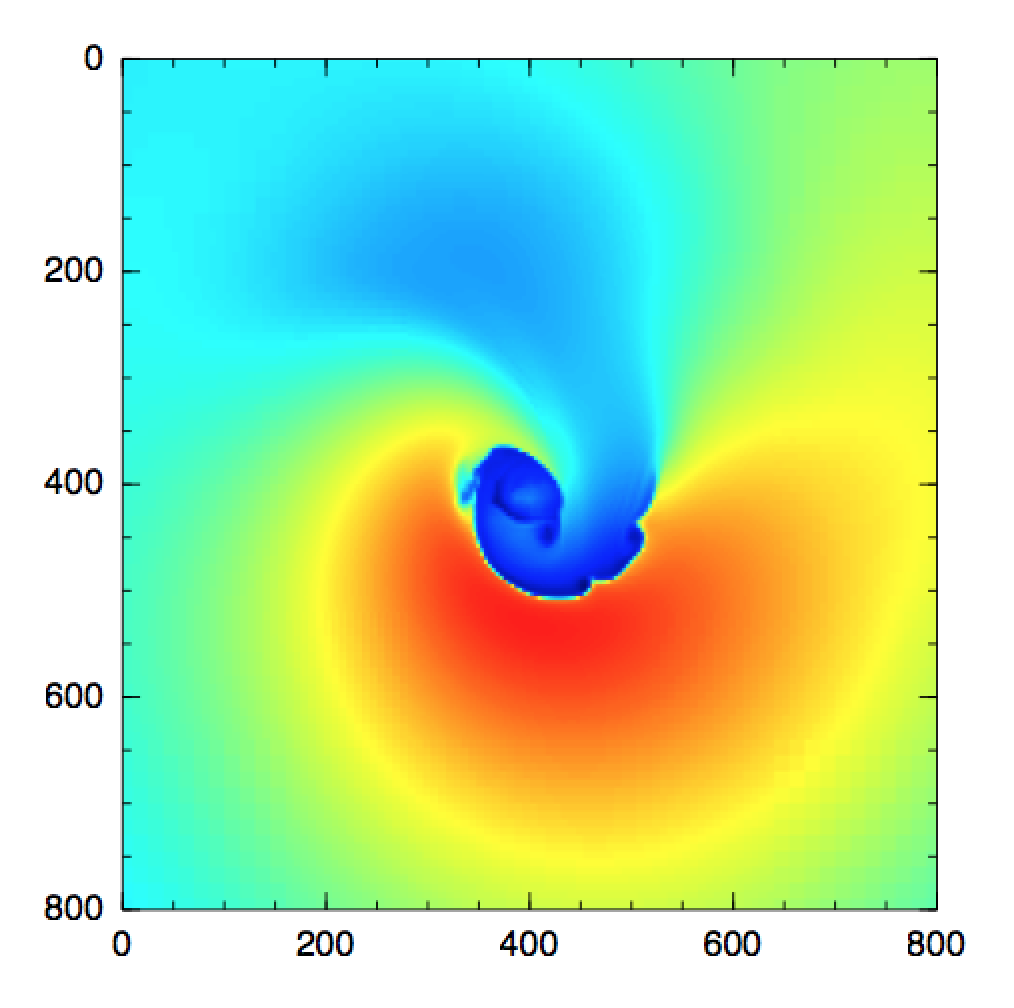
julia> using Winston

julia> imagesc(frb["kT"].value)
which yields the following image: