Profiles
yt allows for data container objects to be binned up into profiles along some dimension defined by a field. These can be in 1D, 2D, or 3D. YT reproduces this functionality via the YTProfile type:
function YTProfile(data_source::DataContainer, bin_fields, fields;
                     n_bins=64, extrema=nothing, logs=nothing,
                     units=nothing, weight_field="cell_mass",
                     accumulation=false, fractional=false)
YTProfile takes the following arguments:
- data_source: The DataContainer object containing the data from which the profile is to be created.
- bin_fields: An Array of field names over which the binning will occur. The number of fields decides whether or not this will be a 1D, 2D, or 3D profile. If a single field string is given, it assumed to be 1D.
- fields: A single field or list of fields to be binned.
- n_bins: A single integer or tuple of 2 or 3 integers, to determine the number of bins along each dimension.
- extrema: A dictionary of tuples (with the field names as the keys) that determine the maximum and minimum of the bin ranges, e.g. [“density”=>(1.0e-30, 1.0e-25)]. If a field’s extrema are not specified, the extrema of the field in the data_source are assumed. The extrema are assumed to be in the units of the field in the units argument unless it is not specified, otherwise they are in the field’s default units.
- logs: A dictionary of tuples (with the field names as the keys) that determine whether the bins are in logspace or linear space, e.g. [“radius”=>false]. If not set, the take_log attribute for the field determines this.
- units: A dictionary of tuples (with the field names as the keys) that determine the units of the field. If not set then the default units for the field are used.
- weight_field: The field to weight the binned fields by when binning. Can be a field name or nothing, to produce an unweighted profile. "cell_mass" is the default.
- accumulation: If true, the profile values for a bin n are the cumulative sum of all the values from bin 1 to n. If the profile is 2D or 3D, an Array of values can be given to control the summation in each dimension independently.
- fractional: If true, the profile values are divided by the sum of all of the values.
For example, to construct a 1D radial profile from a Sphere, with the bins in linear space and with the units of the radius in kpc:
julia> sp = YT.Sphere(ds, "max", (1.0,"Mpc"))

julia> units=["radius"=>"kpc"]

julia> logs=["radius"=>false]

julia> fields=["density","temperature"]

julia> profile = YT.YTProfile(sp, "radius", fields, n_bins=100, units=units, logs=logs)
The bin_fields can be accessed from the YTProfile object as attributes, e.g.:
julia> profile.x
100-element YTArray (kpc):
   4.99991
  14.9997
  24.9995
  34.9993
  44.9992
  54.999
  64.9988
  74.9986
  84.9984
  94.9982
  104.998
  114.998
  124.998
    ⋮
  884.983
  894.983
  904.983
  914.983
  924.983
  934.982
  944.982
  954.982
  964.982
  974.982
  984.981
  994.981
where the attributes x, y, and z correspond to the bin_fields of 1D, 2D, and 3D profiles. The fields of the profile are accessed in the same way as DataContainers:
julia> profile["temperature"]
100-element YTArray (K):
 4.78287e7
 4.78144e7
 5.55494e7
 5.98079e7
 6.20128e7
 6.41538e7
 6.73181e7
 7.28897e7
 7.67484e7
 7.6859e7
 7.65575e7
 7.60974e7
 7.55863e7
 ⋮
 5.15882e7
 5.16148e7
 5.15205e7
 5.15374e7
 5.15363e7
 5.17031e7
 5.15198e7
 5.1652e7
 5.16727e7
 5.17993e7
 5.18381e7
 5.1944e7
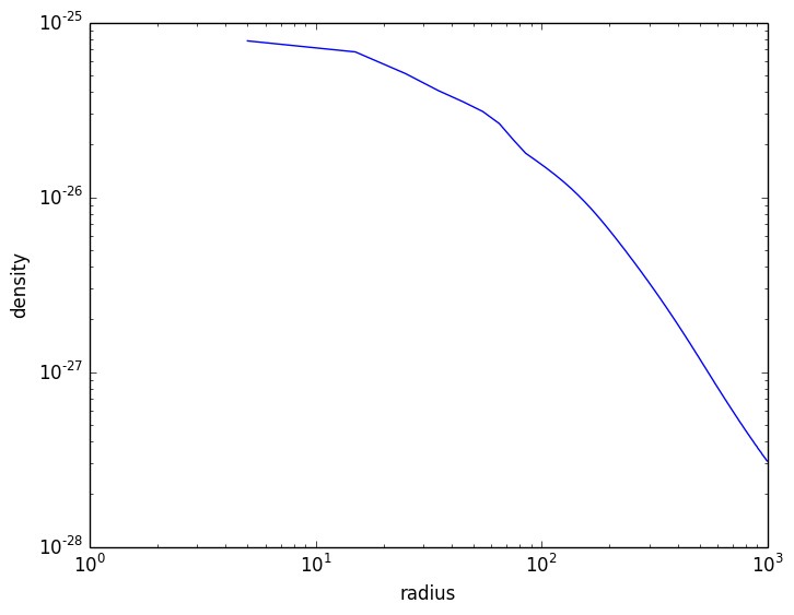
The resulting profile data can be plotted with a plotting program like PyPlot or Winston:
julia> using PyPlot

julia> plot(profile.x.value, profile["density"].value)

julia> xscale("log")

julia> yscale("log")

julia> xlabel("radius")

julia> ylabel("density")
The variance of a given field can be computed as well:
julia> YT.variance(profile, "density")
100-element YTArray (g/cm**3):
 8.88606e-27
 1.00439e-26
 1.05204e-26
 7.17655e-27
 7.2972e-27
 8.29273e-27
 7.97938e-27
 5.74176e-27
 3.73228e-27
 3.28493e-27
 2.91421e-27
 2.58537e-27
 2.27903e-27
 ⋮
 1.28528e-28
 1.28161e-28
 1.25986e-28
 1.25587e-28
 1.24444e-28
 1.24095e-28
 1.21943e-28
 1.21903e-28
 1.20435e-28
 1.20124e-28
 1.18991e-28
 1.18264e-28
The units of the bin_fields can be changed using one of the set_x_unit, set_y_unit, or set_z_unit methods:
julia> YT.set_x_unit(profile, "Mpc")

julia> profile.x
100-element YTArray (Mpc):
 0.00499991
 0.0149997
 0.0249995
 0.0349993
 0.0449992
 0.054999
 0.0649988
 0.0749986
 0.0849984
 0.0949982
 0.104998
 0.114998
 0.124998
 ⋮
 0.884983
 0.894983
 0.904983
 0.914983
 0.924983
 0.934982
 0.944982
 0.954982
 0.964982
 0.974982
 0.984981
 0.994981
Similarly, the units of the fields can be changed with set_field_unit:
julia> YT.set_field_unit(profile, "density", "Msun/kpc**3")

julia> profile["density"]
100-element YTArray (Msun/kpc**3):
 1.16056e6
 1.00365e6
 754309.0
 602161.0
 519959.0
 457351.0
 390482.0
 315199.0
 264284.0
 238734.0
 217263.0
 198420.0
 181572.0
 ⋮
 5663.04
 5563.15
 5426.81
 5324.81
 5220.5
 5140.14
 5011.73
 4930.84
 4834.15
 4757.82
 4663.7
 4584.25